Electronic friction models
To perform molecular dynamics with electronic friction (MDEF) with a specific type of model must be used that provides the friction tensor used to propagate the dynamics. For this, we recommend using FrictionProviders.jl, however, various analytic models can also be employed.
As described on the MDEF page, we consider two ways to obtain friction values, either from the local density friction approximation (LDFA), or from time-dependent perturbation theory (TDPT), also known as orbital-dependent friction (ODF).
An overview of the functionality implemented in FrictionProviders.jl and NQCModels.jl is provided below:
NQCModels.FrictionModels
NQCModels.jl contains the basic type definitions for friction models designed to be paired with Classical and Quantum models.
Classical friction models
Every Classical friction model should be a subtype of FrictionModels.ElectronicFrictionProvider, which describes anything that can fill a n_atoms * n_dofs square matrix with an electronic friction tensor.
As LDFA models are only expected to fill the diagonals of the electronic friction tensor, LDFA models can be a DiagonalFriction type, which enables the integration algorithms used by a DynamicsMethod to dispatch a Diagonal matrix type for greater computational efficiency.
Density models for LDFA
Our Cube-LDFA implementation takes a .cube file containing the electron density, whereas the ML-LDFA models predict the density directly. In both cases the obtained local density is then used to evaluate the friction.
The model works by fitting the LDA data provided by [2] that provides the LDFA friction coefficient as a function of the Wigner-Seitz radius. When the model is initialised, the LDA data from [2] is interpolated using DataInterpolations.jl with a cubic spline. Then, whenever required, the density at the current position is taken directly from the .cube file and converted to the Wigner-Seitz radius with the following relation:
\[r_s(\rho) = (\frac{3}{4\pi \rho (\mathbf{r_{i}})})^{1/3}.\]
Then, the interpolation function is evaluated with this value for the radius, which gives the LDA friction. Optimally, this would be done via an ab initio calculation to get the electron density, but this model instead uses a pre-computed .cube file to get the density with minimal cost. This makes the assumption that the density does not change throughout the dynamics, or that the surface is assumed to be frozen in place.
This graph shows how we interpolate the LDA data and evaluate the friction coefficient as a function of the Wigner-Seitz radius. 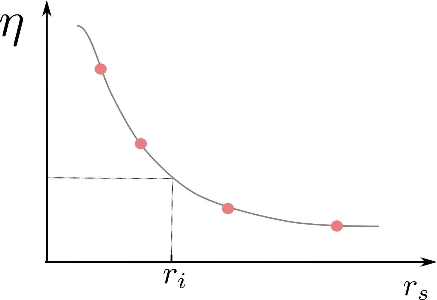
Tensorial Friction models
If a friction model is a subtype of FrictionModels.TensorialFriction, it should provide a full-rank friction matrix with a get_friction_matrix function. NQCModels contains ConstantFriction and RandomFriction models which do this.
Quantum Friction models
Since ab initio friction calculations are often expensive it is useful to have some models that we can use to test different friction methods. The QuantumFrictionModel is the abstract type that groups together the quantum models for which electronic friction can be evaluated. These have an explicit electronic bath, modelling the electronic structure characteristic of a metal. The friction is calculated for these models directly from the nonadiabatic couplings with the equation:
\[γ = 2\pi\hbar \sum_j \langle1|dH|j\rangle\langlej|dH|1\rangle \delta(\omega_j) / \omega_j\]
where the delta function is approximated by a normalised Gaussian function and the sum runs over the adiabatic states ([3], [4]). The matrix elements in this equation are the position derivatives of the diabatic hamiltonian converted to the adiabatic representation.
FrictionProviders.jl
FrictionProviders.jl contains interfaces to machine learning interatomic potentials which predict electronic friction, both for LDFA and ODF.
Currently, FrictionProviders.jl supports LDFA (density) models based on:
- Cube electronic densities
- ACEpotentials.jl
- Scikit-learn
TDPT (ODF) friction models based on:
The use of FrictionProviders.jl with LDFA (Cube calculator and ACE model), and TDPT (ACEds-based model) is explained on the reactive scattering example, to investigate the scattering of a diatomic molecule from a metal surface.