Molecular dynamics with electronic friction (MDEF)
Introduction
A set of fundamental and technologically relevant chemical processes (surface scattering, dissociative chemisorption, surface diffusion, recombinative desorption, etc.) are often catalyzed at the metal surface of several late transition metals (Au, Ag, Cu, Pt, Pd, Rh, etc). These metallic surfaces, unlike other surfaces, are characterized by a dense manifold of electronic states at the Fermi level, which produce continuous conduction and valence bands without a band gap. A theoretical description of the chemical processes at these metal surfaces is often challenging due to the Born-Oppenheimer (BO) approximation no longer being valid. With the breakdown of the Born-Oppenheimer approximation, nonadiabatic effects have to be considered to describe, e.g., the energy exchange that can take place between adsorbate and substrate degrees of freedom (DOF).
A fully quantum dynamical approach of this complex scenario is currently unfeasible and the gas-surface reaction dynamics are often described using quasi-classical methods where nuclear motion is described classically. Molecular dynamics with electronic friction (MDEF) is one of main methods used to deal with the nonadiabaticity in gas-surface chemical reactions. MDEF has been widely employed to decribe and simulate the nuclear dynamics in several molecular systems. It is a theoretical model based on a ground-state Langevin equation of motion which introduces nonadiabatic effects by using frictional and stochastic forces. This approach was originally introduced by Head-Gordon and Tully and the nonadiabatic effects can be included through different electronic friction models (see section below, LDFA and TDPT). The nuclear coordinates of the adsorbate atoms evolve as follows:
\[\mathbf{M}\ddot{\mathbf{R}} = - \nabla_R V(\mathbf{R}) + \mathbf{F}(t) - \Gamma(\mathbf{R}) \dot{\mathbf{R}}\]
The first term on the right hand side of the equation corresponds to a conservative force associated with the potential energy surface (PES) as in the adiabatic case. The third term is the friction force and it comes from multiplication between the electronic friction object ($\Gamma(\mathbf{R})$) and the velocity. Finally, the second term is a temperature and friction-dependent stochastic force which ensures detailed balance.
This figure shows an atom moving near a metal surface $M_A$. When the atom moves into the region of electron density $\rho_0^{M_A}$ it experiences the forces described above. 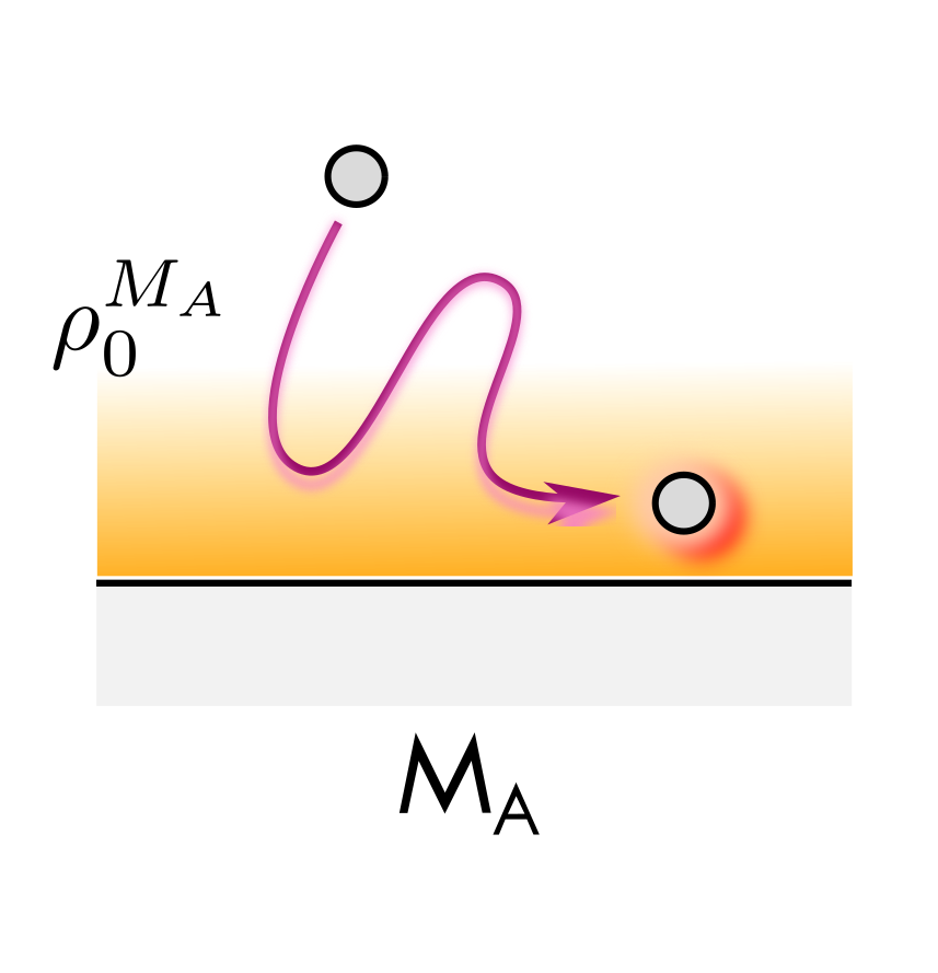
Simple example
We can explore the MDEF concept first by introducing a model system with non-physical parameters. This will demonstrate the general format and expected results from an MDEF simulation which can explore further in later sections using realistic systems.
Here, we model a single hydrogen atom in a harmonic potential, where the electronic temperature is 300 K. The CompositeFrictionModel allows us to combine any ClassicalModel with an ElectronicFrictionProvider that will add electronic friction to an otherwise adiabatic system. RandomFriction is used for demonstration purposes only and provides a matrix of random numbers to use in place of the friction.
using NQCDynamics
using Unitful

atoms = Atoms([:H])
model = CompositeFrictionModel(Harmonic(dofs=3), RandomFriction(3))
sim = Simulation{MDEF}(atoms, model; temperature=300u"K")
Simulation{MDEF{Matrix{Float64}}}:
Atoms{Float64}([:H], [1], [1837.4715941070515])
CompositeFrictionModel{Harmonic{Float64, Float64, Float64}, RandomFriction}(Harmonic{Float64, Float64, Float64}
m: Float64 1.0
ω: Float64 1.0
r₀: Float64 0.0
dofs: Int64 3
, RandomFriction(3))For simplicity, we initialise the system with zero velocity and position for each degree of freedom:
z = DynamicsVariables(sim, zeros(size(sim)), zeros(size(sim)))ComponentVector{Float64}(v = [0.0; 0.0; 0.0;;], r = [0.0; 0.0; 0.0;;])With these parameters, we can run a single trajectory and visualise the total energy as a function of time.
using Plots

solution = run_dynamics(sim, (0.0, 100u"fs"), z, dt=0.5u"fs", output=OutputTotalEnergy)
plot(solution, :OutputTotalEnergy)
:hamiltonian in the output tuple refers to the classical Hamiltonian that generates the classical equations of motion. Since we are performing MDEF we see that the total energy fluctuates.
Now let's see what happens if we make the electronic temperature a function of time. For any simulation, temperature can be provided as a time-dependent function which allows variable temperature simulations. In the context of MDEF, this temperature can be used to represent the use of lasers to provide extra energy to the electrons in the metal.
temperature_function(t) = exp(-(t - 50u"fs")^2 / 20u"fs^2") * 300u"K"The time argument enters this function as a Unitful.jl quantity, and it is important to make sure the unit of the return value is temperature.
Now we can re-simulate, replacing the fixed temperature with the function we have defined.
sim = Simulation{MDEF}(atoms, model; temperature=temperature_function)
solution = run_dynamics(sim, (0.0, 100u"fs"), z, dt=0.5u"fs",
    output=OutputTotalEnergy)
plot(solution, :OutputTotalEnergy)
This time we see a peak in the energy in the middle of the simulation which coincides with the peak in temperature at 50 fs. Having viewed this simple example, we can now explore the different ways the friction coefficient can be obtained from ab initio simulations.
Local density friction approximation (LDFA)
Local density friction approximation (LDFA) is a theoretical model which describes the electronic friction $\Gamma(\mathbf{R})$ term in the above equation based on the local electron density of the metal substrate. This approximation assumes a scalar friction coefficient ($\Gamma(R_i)$) for each adsorbate atom. The underlying assumption to this approximation is that any atom only sees an anisotropic (scalar) density that only depends on the local surroundings. In the LDFA theoretical framework the above equation of motion is used, except the friction matrix is diagonal, each element coming from the local density of each atom.
In our current LDFA implementation, a set of pre-calculated electronic friction coefficients ($\eta_{e,i}$) computed at different Wigner-Seitz radius ($r_s$) are used to fit and get an analytical expression to connect any $r_s$ values with an single electronic friction coefficient by means of cubic Spline functions. The Wigner-Seitz radius is connected to the metal substrate electron density by the following equation,
\[ r_s(\rho) = (\frac{3}{4\pi \rho (\mathbf{r_{i}})})^{1/3}\]
In this way, the electron density associated with the current substrate atom position is used to compute the respective friction coefficient through fitting function for each point of the trajectory. Visit the FrictionProviders.jl to learn more about how this is evaluated.
Time-dependent Perturbation theory (TDPT)
A more general formulation of the electronic friction object was also developed under the umbrella of electronic friction tensor(EFT) or orbital-dependent electronic friction (ODF) approaches. Both formulations are essentially equivalent and they incorporate the isotropy nature of the electronic friction object by a multidimentional tensor ($\Lambda_{ij}$) instead of a single coefficient as usually computed at LDFA level. The electronic friction elements can be computed by first-principle calculations in the context of first-order time-dependent perturbation theory (TDPT) at the density functional theory (DFT) level. Each electronic friction tensor (EFT) elements corresponds to relaxation rate due to electron-nuclear coupling along the Cartesian coordinate $i$ due to motion in the $j$ direction. The electronic friction tensor elements can be computed by using the Fermi's golden rule. $\Lambda_{ij}$ is an object with ($3N\times3N$)-dimension where N is often the total number of adsorbate atoms considered explicitly on the study system. View the friction models page to learn about how this can be used.
If you would like to see an example using both LDFA and TDPT during full dimensional dynamics, refer to the reactive scattering example.
Use of Composite models for phonon thermostatting
using NQCDynamics
using Unitful, UnitfulAtomic
using Plots

# Create an example surface structure
atoms = Atoms(vcat([:H, :H], [:Cu for _ in 1:54])) #define atoms
positions = rand(3,56) # Placeholder for atomic positions, often read in from ASE file

# PES applies to all atoms
pes_subsystem = Subsystem(Free(3)) #Subsystem(pes_model())

# Electronic friction applies to adsorbate atoms 55,56
electronic_friction = Subsystem(RandomFriction(3), [55,56])

# Combine models and generate Simulation
combined_model = CompositeModel(pes_subsystem, electronic_friction)

T_el_function(t) = exp(-(t - 100.0u"fs")^2 / 50u"fs^2") * 500u"K"

sim_T_el_only = Simulation{MDEF}(
   atoms,
   combined_model;
   temperature = T_el_function
)

v = zeros(size(sim_T_el_only))
r = zeros(size(sim_T_el_only))

v[:, 55] = [austrip(5.0u"eV"), austrip(-3.0u"eV"), 0.0]
v[:, 56] = [austrip(2.0u"eV"), austrip(0.0u"eV"), 0.0]
z = DynamicsVariables(sim_T_el_only, v, positions)

solution = run_dynamics(sim_T_el_only, (0.0, 750u"fs"), z, dt=1.0u"fs", output=OutputTotalEnergy)
plot(solution, :OutputTotalEnergy)